Executive Summary
- Market risk, that is to say the variability of returns from one period to the next, or volatility, is one of the many risks faced by investors in equities, bonds and currencies. In the case of U.S. equities, the VIX by the Chicago Board Option exchange (CBOE) measures implied volatility, i.e. the level of volatility implied by the prices of S&P options. It is seen as a forward looking measure, in contrast to realized (or actual) volatility, which measures the variability of historical (or known) prices.
- In this paper, we introduce perceived volatility, an exponential and dynamically-weighted combination of past returns on the S&P 500. We find that it is closely correlated with implied volatility, showing that the VIX may just be a (smart) reflection of the past instead of a real forward-looking measure, as generally claimed.
- Just like implied volatility, perceived volatility has some predicting power of future volatility (27% standard estimation error), but the model is unstable and limited to short forecasting horizons (38-trading day is the optimal forecasting horizon, very close to the VIX promise).
- This matters because volatility — be it historical or implied — is widely used to calibrate risk-taking in the financial services industry, from volatility-targeting strategies, to collateral requirements estimation, to prudential regulation. As such, it is a potential endogenous source of man-made unknown unknowns.
Market volatility: What a maze!
No pain, no gain! No risk, no return! Simple as it is, this basic idea underpins both the theory and the practice of investing. But what is risk and how should it be measured? Investment risk is a hydra that manifests itself in different ways. For instance, the buyer of a corporate bond may or may not get in due time all the money owed to him by the issuer — this is credit risk. Similarly, the owner of a stock may or may not find it easy to sell her holdings without depressing market prices — this is liquidity risk. The price in a week’s time of a share, a bond or a currency may or may not be very different from today’s price: this is market risk, the subject matter of this paper.
Historical volatility relates to the variability of past returns. For example, in the case of the S&P 500 from January 3rd, 1986 to December 6th, 2019 (i.e. 8,844 equally-weighted daily observations), the average daily (log) return has been 0.03% while its daily standard-deviation has been 1.11%. Had we conducted this exercise on 32 equally-weighted annual observations, we would have found that the average annual return has been 7.98%, while its annual standard-deviation has been 15.63%. That the historical daily volatility of the S&P 500 has been 1.11% over the last 33 years (or 15.63% at annual rate) may be a valuable statistical observation for an historian. But what matters to an investor is the volatility of returns over the next 30, 90, 180 days … depending on his investment horizon. How confident can he be that the past is any guide to the future?
Now, hardly a day or a week goes by without pundits suggesting that the CBOE’s Vix index captures U.S. equity market risk. When they do bother to define this index, they are content with repeating - time and again - how conventional wisdom claims the Vix should be interpreted. To wit:
“Wall Street’s so-called fear gauge […], the CBOE’s Vix index, […] gauges investor expectations of short-term volatility in US stocks. The Vix index is the most closely watched gauge of implied volatility in the world’s biggest stock market. It reflects the cost of buying short-term options on the S&P 500”;
or, from other recent example:
“The Vix volatility index – a measure of expected swings in the S&P over the next 30 days – has slumped to 12.78, not far off its lowest levels of the year, and well below its 30-year average of around 19.”
To be fair, prominent practitioners lend their credibility to such statements. To wit:
“Implied volatilities are used to monitor the market’s opinion about the volatility of a particular stock. Whereas historical volatilities are backward looking, implied volatilities are forward looking.” ;
Another example:
“[Implied volatilities] are based on prevailing market prices rather than on the past history of returns and, therefore, they are forward-looking measures of volatility.”
These four statements create a kind of maze of seemingly important concepts: backward looking historical volatilities, forward-looking implied volatilities, volatility index, investor expectations of short-term volatility and Wall Street’s fear gauge.
How to walk through this maze, how to connect these dots, is the subject matter of the present investigation. We will start by defining historical as well as implied volatility. We will then argue that implied volatility is not as forward-looking as generally believed. Provided historical returns are properly weighted, implied volatility is indeed strongly correlated with historical volatility. Furthermore, the causality runs both ways, from implied to historical volatility, but also the other way around. This calls into question the basis of some of the most closely watched barometers of market uncertainty, and has consequences for and volatility-targeting strategies.
Historical volatility is...volatile
The essential characteristic of the daily, weekly, monthly… historical (or past) returns on bonds and equities is that they are not constant through time. They can be positive or negative, and more or less so in either direction. In other words, they are volatile. In first approximation at least, the distributions of historical asset returns are close to the famous bell-curve distribution, with a large bump in the middle and progressively thinner and thinner symmetric tails on either side.
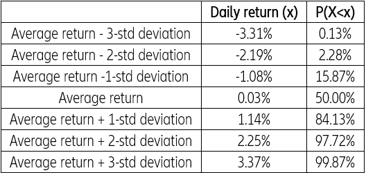
At the center of the distribution lies the average historical return; the larger the absolute deviation from the average return, the lower its frequency. Under the controversial assumption that empirical distributions follow the bell-curve pattern, one single statistical parameter – the standard-deviation of returns – suffices to characterize the dispersion of returns around their average, as shown in Table 1 In finance, the standard deviation of historical returns is called historical volatility. On it depend both the range and the frequency of potential outcomes.
However, historical volatility is easier to define than to measure. Measuring historical volatility would be simple if it did not depend on the observations selected to estimate it. Unfortunately, historical volatility itself is volatile: the volatility observed during the last three weeks, months or years is generally not the same as the one observed during the three previous or the three subsequent weeks, months or years. Therefore, an analyst looking to measure historical volatility must decide, first, which set of past returns is relevant in the case of interest and, second, how to weight those past returns. Needless to say, answering these two questions is more an art than a science. While pondering various alternatives, an analyst should bear in mind two additional stylized facts that characterize the (mis)behavior of financial markets:
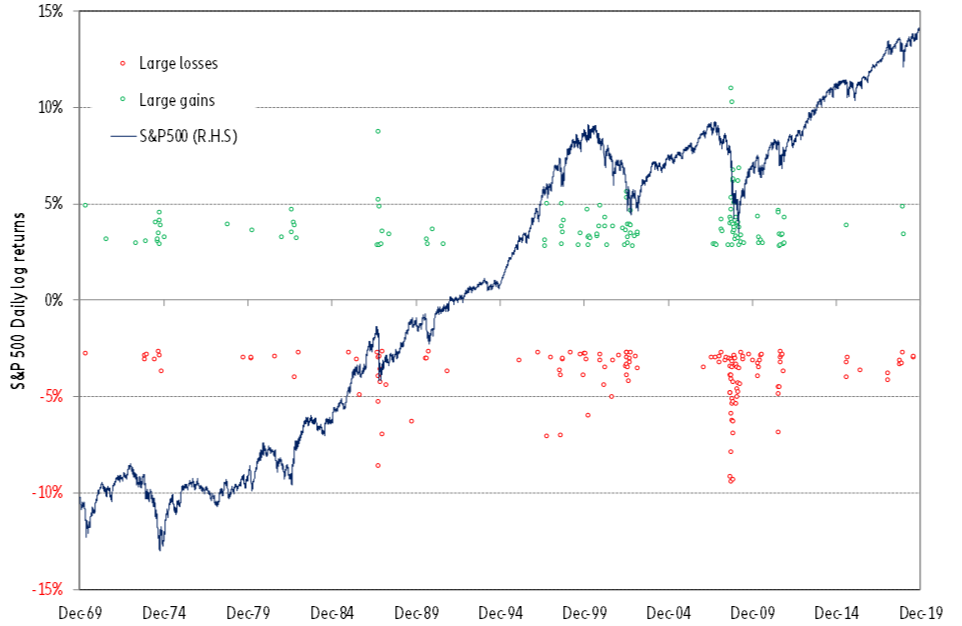
- large returns - be they positive or negative - are not uniformly distributed through time, but tend to cluster at irregular time intervals
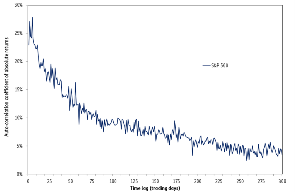
while there is only negligible dependence between consecutive returns, there is a significant degree of autocorrelation between lagged squared or absolute returns
In plain English, large - positive or negative - absolute returns tend to be followed by other large - positive or negative - absolute returns, so that when volatility becomes volatile it tends to be persistently so. In the case of the S&P 500, Figure 1 illustrates the first two of these stylized facts; Figure 2, the last one.
Altogether, these stylized facts point to an alternation of periods of low and high volatility, as well as to persistent trends in volatility. As such, they call for an agile technique to monitor volatility, a technique that can quickly capture regime changes, while smoothing out the short-term noise. Such a compromise is achieved by giving historical returns weights that depend on how recent they are, so that the weights decrease as we move back through time.
The case for perceived volatility as a way to track historical volatility
This kind of declining weighting scheme is a common feature of the three standard ways to track volatility: the exponentially weighted moving average (EWMA), Autoregressive Conditional Heteroskedasticity (ARCH) and Generalized Autoregressive Conditional Heteroskedasticity (GARCH) models. In the EWMA model, weights decline exponentially at a constant rate that one needs to optimize on a given data sample (see Appendix I). The ARCH and GARCH models are somewhat more flexible than the EWMA model as the weights do not decline at a constant rate: they are directly estimated, but here again their optimization is dependent on a given data sample. In these three types of models, as the weighting structure depends on a given data sample, it is always liable not to be optimal when applied to fresh out-of-sample data.
In contrast to these three techniques, the Allais transformation relies on an embedded dynamic mechanism to deal with regime changes (see Appendix I). Admittedly, Allais did not design this algorithm to measure the historical volatility of asset returns. But the statistical characteristics of those returns (non-stationarity, volatility clusters, autocorrelation of squared or absolute returns) make it ideally fit to do so. Hence, we use this transformation to compute what we shall henceforth call perceived volatility to distinguish it from usual measures of historical volatility (like EWMA, ARCH, GARCH). Since perceived volatility is backward-looking or path-dependent, it is one metrics of historical volatility. To this extent, the word “perceived” is synonym of the word “historical”. In the presence of increasingly large absolute returns, Allais’s transformation gives an increasing weight to the most recent absolute returns, the relative change in the weights depending on the magnitude of the latest surprise or forecast error. In an uncertain world, a world of unknown unknowns, such a weighting scheme potentially provides an accurate description of how we imagine the future by learning from past experience. If that is the case, backward-looking as it may be, perceived volatility should shed light on how options are priced. The volatility “expected” by market participants is indeed “the” critical variable, not to say the joker, in Black and Scholes’s option pricing model.
Implied volatility is nothing but the solution of a reverse-engineering problem
Like any asset pricing model, the famous Black and Scholes’s option pricing model is a two-way street. A set of input variables being given, its primary function is to compute the theoretical price of an option. But, through a reverse-engineering exercise, it can also be used to compute the value of an input variable that is consistent with or rather implied by the market price of an option. The expected volatility of an asset’s returns being one of Black and Scholes’s model input variables, implied volatility is the value of expected volatility that is implied by the market price of an option on this asset (see Box).
THEORY BOX
The buyer of an option has the right to buy (call option) or to sell (put option) an underlying asset, on a certain date (European option) or at any time until a certain date (American option), at a given price (the strike price).
According to the Black and Scholes formula, the price of an option is a function of four directly observable variables:
The strike price of the option
The current price of the underlying asset
The time remaining to the expiry date of the option
The risk-free rate of interest
and one variable that is not directly observable, the expected volatility of the underlying asset. Because it is not directly observable, it is the genuine price of an option; it reflects a market consensus.
In the case of a call, the more the current price of the underlying asset exceeds its strike price, the greater the price of the option. For both calls and puts, the more time that remains until the expiry date or the greater the volatility of the underlying asset, the more things may happen, hence the greater the price of the option. Finally, the lower the risk-free rate, the greater the present value of all possible outcomes, hence the greater the price of the option.
In this framework, volatility is meant to be forward-looking, to be a forecast. It is not meant to depend on historical volatility.
As volatility is not directly observable, two types of “what if” questions may be raised:
The straight question: what is the theoretical price of an option for a given level of expected volatility?
The reverse question: what is the level of volatility implied by the market price of a given option?
The answer to this second question is called “implied volatility”.
However, implied volatility has to be revealed to the layman by geeks who use complex mathematical formulae to extract information from market prices. It is therefore both mysterious and intimidating. By the leap of faith that markets are efficient, implied volatility is interpreted as a forward-looking indicator of market volatility.
If this forward-looking interpretation is correct, implied volatilities should be valuable inputs in internal risk models to ex ante calibrate risk-taking. This probably explains why implied volatility indices are computed on a daily basis for all major options markets, the oldest one being the VIX, calculated by the CBOE since 1986 for options on the S&P100 equity index. The VIX is actually an average of one-month implied volatilities for various strikes, for puts as well as call options. But how confident can we be that implied volatility is a forward-looking expectation? Backward-looking expectations being present in the pricing of other financial instruments, like long-term bonds, why should they be totally absent from option pricing?
Implied volatility is closely linked to perceived volatility
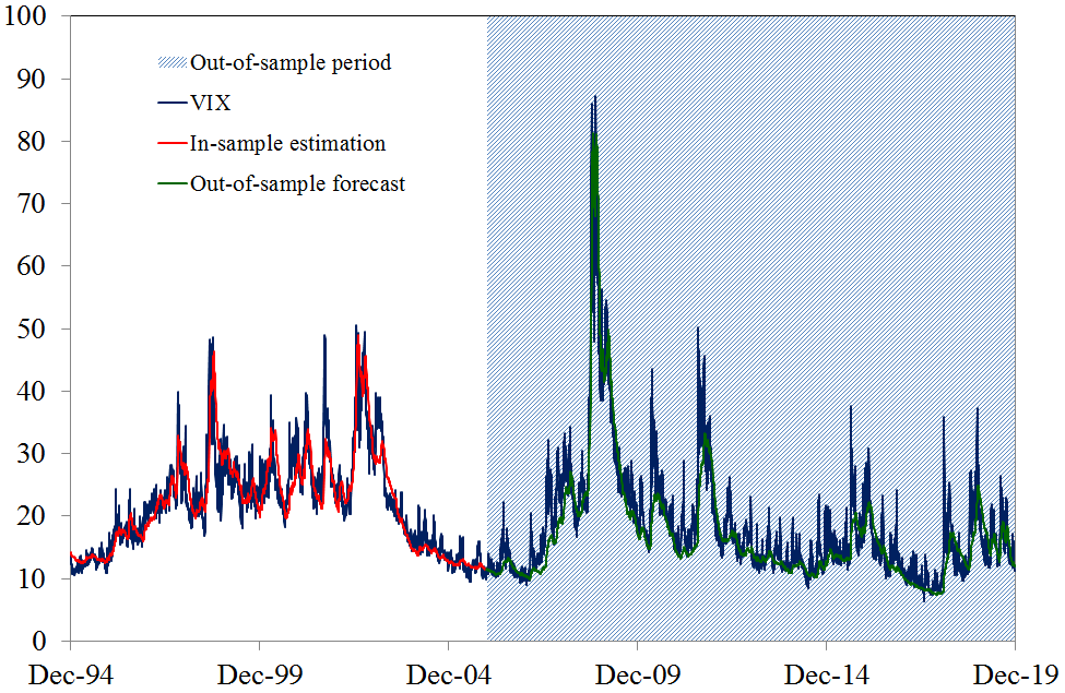
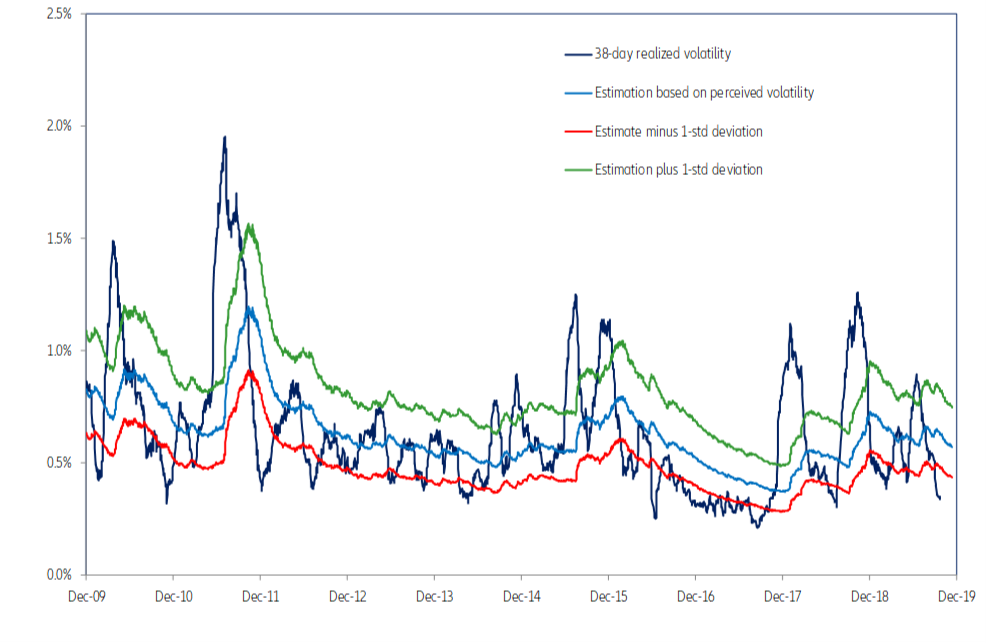
Like it or not, Figure 3 shows that implied volatility and perceived volatility have been closely correlated (see model 1 in Appendix II), both in-sample (from 15/07/1993 to 30/12/2005) and out-of-sample (from 30/12/2005 onwards).
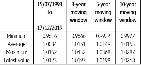
In other words, the path followed by past returns, which is captured by perceived volatility, does fit in with implied volatility or, more simply, past returns are present in implied volatility. Most interestingly, this relationship is a reliable one, as the model’s key coefficient is very stable (see Table 2).
But correlation does not necessarily imply causation in any meaningful sense of that word: correlations may be spurious or meaningless. To test whether perceived volatility “causes” implied volatility, the Granger causality test first computes how much of the current implied volatility can be explained by its past values. It then tests whether adding lagged values of perceived volatility can improve the explanation. If that is the case, perceived volatility is said to cause implied volatility. As interdependence is ubiquitous in economics and finance, two-way causation happens to be frequent. Granger causality measures precedence and information content but does not by itself indicate causality in the more common sense of the term. The result of Granger causality test depends, of course, of the lag used.
For lags of one to five days, two-way causation prevails between perceived and implied volatility. Then for lags of six to eight days, the causality runs from implied volatility to perceived volatility by a wide margin. Beyond nine days, there is no clear pattern. That implied volatility may sometimes lead perceived volatility by a few days is confirmed by the fact that it is possible improve the accuracy of the first model by introducing an eight-day lag between the two variables. However, the improvement is quite marginal. In plain English, all this means three things:
- first, perceived and implied volatilities very much tell the same story, the past is present in the present: once bitten, twice shy!
- second, conventional wisdom notwithstanding, there is some evidence that implied volatility is backward-looking.
- third, in financial markets, people tend to buy insurance once an accident or a catastrophe has occurred, but not before.
Perceived volatility (alias implied volatility) is not indicative of future volatility
Does this mean that perceived volatility or implied volatility are of no use to forecast future volatility? Not necessarily, owing to the three stylized facts mentioned above (alternation of different volatility regimes, volatility clusters, autocorrelation of absolute or squared returns).
As a matter of fact, there is some correlation between perceived volatility and future volatility: it is not very high, it varies with the forecasting horizon, which is in any case rather short, but it is there. This is what a model having the structure of the second one does show. Why use perceived rather than implied volatility as an input in this model? Because perceived volatility can be computed as far back as asset prices are available, while implied volatility time series only start when options markets were created. In the case of the S&P 500, from January 1970 to December 2006, the highest correlation is obtained over a 38-trading day forecasting horizon (almost eight weeks). However – even on this optimal forecasting horizon – the R-SQ is only 47%, the standard estimation error is 27% of future volatility (i.e. about 3 points of annualized volatility) and the model is not particularly stable out-of-sample. At the current juncture, its suggests that future volatility should be rising (Figure 4).
But it would not be reasonable to bet the ranch on such a model. At the risk of borrowing the famous line according to which past performance is not indicative of future returns, one could say that neither implied volatility nor its kin - perceived volatility - is indicative of future volatility. So what? Does it matter? And if so, why?
Beware of future volatility
It does matter for at least four reasons. First, because – as shown in Figure 3 - volatility can be very volatile (from 1994 to date, it has fluctuated between the low tens and 90%). Second, because – as shown in Figure 1 – volatility tends to increase when markets crash. This is why when a practitioner boldly “predicts” that a market will be volatile, the layman should decipher such a statement as a forecast that prices will fall. Third, because the financial services industry pervasively uses volatility – be it historical or implied – to calibrate the size of its positions – be they long or short – notwithstanding the fact that future volatility is hard to predict. Fourth, because volatility spikes are liable to stress money markets through collateral and margin calls.
A case in point are those strategies that systematically sell options (i.e. implied volatility) to enhance returns in a low interest rate environment (so-called “inverse volatility” strategies). The hunt for yield fostered by unconventional monetary policy is indeed incentivizing investors, even retail ones, to sell options. The more the central banks’ “puts” are credible, the greater the incentive to write slightly out-of-the-money options so as to cash in the corresponding premiums, hoping the options will not be exercised.
This increased supply of implied volatility tends to compress implied as well as realized volatility most of the time, but it also fosters by the same token the brutal volatility spikes seen in early and late 2018. Through a second-round cumulative effect, the low level of volatility is indeed an incentive to take more risk in the many volatility-targeting strategies – like risk-parity strategies or Solvency II ratios – that rely on the ubiquitous Value-at-Risk (VaR) models. This initially directly supports the prices of the underlying assets. All the resulting positions are easy to price and to manage as long as the prices of the underlying assets move, if not continuously (as assumed in the Black & Scholes model), at least gradually.
But this is by design an unstable equilibrium. In February 2018, in one single trading day, an “inverse volatility” exchange-traded product lost 90% of its value. As a matter of fact, large price gaps (discontinuities) can trigger a chain reaction of cumulative, self-reinforcing, forced selling. This is what happened with “portfolio insurance” in October 1987, following a large downward move triggered by some unexpected “bad news”: to limit their potential losses, equity put sellers became forced sellers of equity futures, thus reinforcing the vicious positive feedback loop they were trying to escape. In other words, risk is not a kind of physical constant that Nature would “give” to a market; it is man-made, it is endogenous to markets.
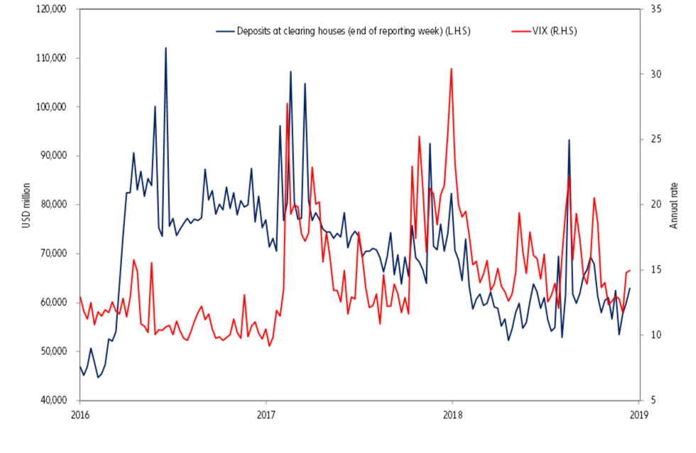
Following the Great Financial Crisis, to alleviate the credit risk present in derivatives transactions, they are increasingly being settled through clearing houses and secured by collateral and margin calls. As a result, volatility spikes do have an impact on the demand for liquidity. In the last two years, as shown in Figure 5, we have experienced three brutal rises in the VIX: the first, in January 2018; the second, from October to December 2018; the third, in July-August 2019. In all three cases, the deposits made at clearing houses rose significantly. In the last instance, the overnight repo rate briefly rose to 10%, 775 basis points above the Federal Funds target rate!
As Hyman Minsky put it, “stability begets instability”. This aphorism is never so true and worth remembering as when volatility has been low for a long time.


